VSTACK Function: Combine Multiple Sheets into One Array

SUMMARY

March 2022 saw the release of 14 new Excel functions specifically for working with text and dynamic arrays. Use these functions to split text or combine, resize, and reshape arrays. VSTACK uses the dynamic array environment to combine lists and arrays vertically into a single array.

Objectives:

• Define the VSTACK and HSTACK Formula and Benefits
• Create Clean Data with Which to Work
• Create Tables from your Data
• Use the VSTACK function to combine data from multiple sheets (arrays)
• Create a Dynamic Pivot Table using the newly created worksheet

What are VSTACK and HSTACK in Excel?

VSTACK and HSTACK (New in 2022) help you to easily combine multiple lists into one list in Excel. Stacking, or appending, tables and lists on top of or next to each other can now be done more easily. No need to alter your original data or use complex nesting and intermediate-to-advanced tools  Power Query Add-in is a method you can use for automatic updates, however.

Create a Table from Your Clean Data

It’s best to create a table for use with Reports, Dashboards and Pivot Tables. While you may think that this is unnecessary and time-consuming, I promise it will save you headaches and time in the end. You will also enable additional features for Pivot Tables and Pivot Charts if you create a table from your data. (More later!)

1. Ensure your Data is properly prepared.
   • No blank lines or columns.
   • Headers above every column.
   • Data is separated from superfluous data such as Titles.
2. Select Data.
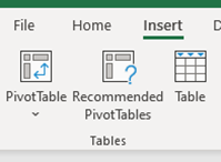
3. Insert–Tables Group–Tables

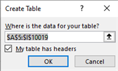
The Create Table Dialog Box appears.

4. Confirm Range.
5. Confirm whether or not your table has headers
6. Choose OK.

7. Name Your Table
8. Table Design–Properties–Table Name
9. Type the Table Name

Add VSTACK Formula

On a worksheet named Vstack, I created an Excel spill formula in cell A1:

=VSTACK(TBLJanSales[#All],TBLFebSales,TBLMarSales)

That formula returns a vertical stack from the contents of 3 ranges:

1. Headers and data from TBLJanSales
2. Data from TBLFebSales
3. Data from TBLMarchSales

All 3 ranges have the same number of columns, but different numbers of rows.

1. Select Cell where combined range will begin (I used A5)
2. Type =VStack

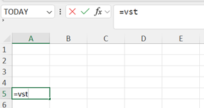
3. Double Click on VStack in Contextual Menu to insert it in Formula Bar

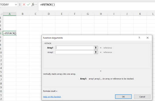
4. Click the FX button to open the Function Arguments Dialog Box

5. Select headers and data from January sheet “TBLJanSales” for Array 1
6. Select ONLY the data from the February Sheet “TBLFebSales for Array 2
7. Select ONLY the data from the March Sheet “TBLMarch” for Array 3

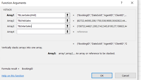
8. Click OK

Name Combined Data Range

¡IMPORTANT!

To use the combined data as a pivot table source, it’s important to create a named range, based on the VSTACK formula cell.

1. On the VStack sheet, select cell A5 (Or whatever cell you placed the VSTACK function)
2. Formulas–Defined Names–Define Name
3. In the name box, type “PIVOTDATA”
4. In the Refers to box, where the address is showing, type a number sign at the end: =VStack!$A$1#

This creates a reference to the cell’s spill range — all the “spill” cells with the combined data.

5. Click the OK button, to complete the name

Create a Pivot Table

1. Select cell A5 (Or whatever cell you just named with the VSTACK function) or somewhere in data range
2. Insert–Table–Pivot Table
3. When the Pivot Table from table or range dialog box opens, clear the Table/Range box
4. Type the defined name that you created, e.g. PivotData
5. Click the OK button
6. From PivotTable Field List add fields to the pivot table layout (For this example I used Agent ID in Row Area and Amount in Values Area)
7. Rename and Format Pivot Table as you normally would

Phew!  Did that work?  Let me know.  I love this function, but I don’t get to show it to people as much as I’d like because of our short workshops.  What do you think?  Will it work for you?

¡IMPORTANT!

These functions will return an ARRAY. You may not alter (delete, move copy, etc.) any part of an array, therefore if you want to manipulate the data simply copy it and use Paste Special to paste it as a value.

There you have it! Some great ways to save time and frustration by using Excel’s Autofill feature. How can you get even more creative after trying these techniques? Let me know, I’d love to hear from you. Until then, Have an EXCEL-LENT day!!–Stephanie