 Arena Training
 This article assumes that one knows the basics of PivotTables and Conditional Formatting. For a Conditional Formatting Tutorial, Click HERE.
Why Use Conditional Formatting?
Using conditional formatting adds life and clarity to your Excel Table. Formatting cells to stand out from the table helps it to be impactful and easy to understand. You can set rules to format cells based on the criteria you choose so that the formatting is applied automatically.
PivotTables are dynamic. Each time the source data is updated; so will your Table. How do you update the conditional formatting as well?
In this example we manage conditional formatting to do just that; saving you time and frustration when the Table updates.
Use Conditional Formatting Dynamically
Using the conditional formatting feature with a PivotTable in Excel is just a little different than for ranges outside a PivotTable. That’s because the PivotTable data source changes and we must let Excel Know to update these changes.
Let’s Try it!
You can use your own PivotTable or download my sample from below. We will conditionally format all values (Revenues) for 2020 over $500,000 to be displayed in yellow background with dark yellow text. Of course, you can choose other formatting. This is for the sake of simplicity to understand the concept.
- Select ONE cell in the values area of the PivotTable that you wish to format.
- Choose Home→Styles Group→Conditional Formatting→Highlight Cell Rules→Greater Than
- In the Format cells that are GREATER THAN Box, Enter 500000.

- In the Formatting Box→Click the Drop-down arrow and choose a format. (I chose the yellow fill) →Choose Ok.
NOTE: This is where conditional formatting differs a bit when using a PivotTable. Since you only selected one cell; only one cell is highlighted. We need to fix this.
Notice a “Formatting Options” Button appeared beside the cell that has the conditional formatting applied. You will use this to provide Excel other options for formatting.
- Click on the formatting options button. Note the menu. (Go to ** below if you cannot see the formatting options button)

- Select the 3rd option. WHY? You do not want to include the GRAND TOTAL in the conditional formatting rule. That would not make sense. Experiment—it will make sense.
- Click on the Drop-down arrow beside (ALL) and filter only for 2021. Note Changes.
- Filter for 2020. Note changes update.
Pretty Cool, huh?? 😊
Let me know what you think.
**If you do not see the “Formatting Options” button as displayed above, you can find the options another way.
- Home→Styles Group→Conditional Formatting→Manage Rules
- Select the rule and choose Edit
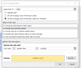
- In the upper section Choose the formatting option (we chose the third to omit the Grand total)