 Arena Training
 Hi there Excel users! Stephanie Hutcheson here. Trying to save the world some headaches.
I frequently get asked to explain how to show leading zeros in Excel. It’s so frustrating when a leading zero drops from your worksheet. While you can format it as text or type an apostrophe in front of it, you may want to consider a custom format that you can reuse on this and other worksheets.
You may know that when you display a number in a specific format, it doesn’t change the underlying value of the number. For example, the number 1000 as 1000 or 1,000 or 1000.00 or 001000 or 26-09-1902 (even dates are numbers in the backend in Excel).
In all the different ways to display the number, the value of the number never changes. It’s only the way it’s displayed that is changed.
To add leading zeroes, we can format it to show it that way, while the underlying value would remain unchanged.
Here are the steps to add leading zeroes in Excel
- Select the cells in which you want to add leading zeroes.
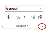
- Home–Number Group–dialog launcher (a small tilted arrow in the bottom right -See Figure 1). This will open the Format Cells dialog box. (You can also press Control + 1).
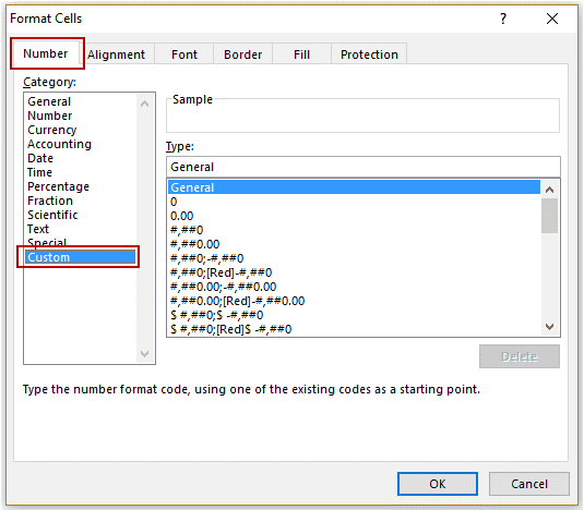
- In the Format Cells dialog box, within the Number tab, select Custom in the Category list.
- Select the choice #,##0 if you want the number to be formatted with a thousand separator, otherwise choose appropriate format or create your own.
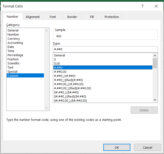
- In the TYPE box, type a 0 in front of the format code as below.
0,#,##0
- Choose OK.
It is automatically saved. That’s it!!
To apply to another cell or cells.
- Select the cell or cells
- Right Click
- Choose format
- Choose Custom
- Find your custom format
Let me know if this works. Leave some of your creative comments below!
Have an EXCEL–LENT DAY!!