 Arena Training
 When you’re not in the mood for change!
Protecting the Workbook Structure
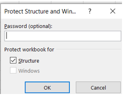
Protecting the workbook structure prevents the user from viewing hidden worksheets, adding, moving, deleting, hiding, or renaming them. You can protect the structure of your Excel workbook with a password if you choose, but it is not necessary.
- Review–Protect Workbook
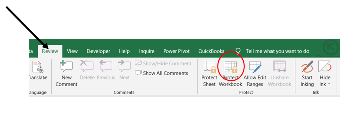
- Choose Protect Workbook
- Password if you choose
- OK
You will be able to add data, but not change the structure as mentioned prior.
Protect the Entire Worksheet from Updates to Data
To protect the worksheet from data updates, you need to Protect the Worksheet, not the Workbook.
- Review–Protect Sheet
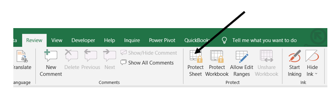
- Password if you choose
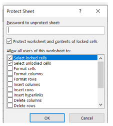
- Select Your Options
- Choose OK
- Test your worksheet by entering data into a cell. You will not be able to enter any data or update formats and will receive a message indicating that your sheet is protected with instructions on how to unprotect it.
Protecting specified data from change in Excel is a two-step process.
Unlocking specific cells permits changes to be made to these cells after the protect sheet option has been applied.
Step one involves locking/unlocking specific cells in your spreadsheet.
Step two involves applying the Protect Sheet option. Until step 2 is completed, all data is vulnerable to change.
As mentioned earlier; by default, all cells in an Excel spreadsheet are locked. This makes it very easy to protect all data in a single worksheet simply by applying the Protect Sheet option as we saw above.
Unlocking specific cells permits changes to be made to these cells after the protect sheet option has been applied.
NOTE: You may need to Unprotect your worksheet if you followed the above tutorial.
Review–Unprotect Sheet; type Password if necessary
Step One: Unlock Cells in Excel
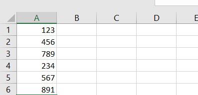
- Enter the following data into cells A1 to A6:
- Select cells A1 and A2.
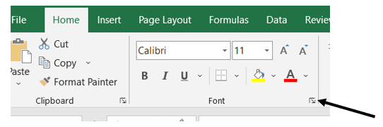
- Click on Home–Font Grouping–Dialog Box Launcher
- Select the Protection Tab
- Click the Lock Cell checkbox to uncheck. (it is probably checked by default)
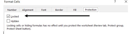
- The Lock Cell option is an ON/OFF button. Since all cells are initially locked in the worksheet, unchecking this option Unlocks the highlighted cells A1 and A2.
Step Two: Protect the Worksheet
- Select the Review Tab to open the Review ribbon.
- Click Protect worksheet
- You may password protect if you like. WARNING!! If you forget your password you are out-of-luck (Unless you have skills. :-0)
- Notice the checkbox reminding you that this will only protect LOCKED CELLS. We unlocked Cells A1 and A2, so this will not affect those.
- Notice you may choose to only protect against certain options. Peruse the list! It may prove useful.
- Choose ok.
Test the Worksheet
- Try changing cell A4 to 123. Can you update the value?
- Try changing cell A1 to 789. Can you update the value?
That should do it!
Hopefully you had some fun with this tutorial. Leave a comment on my website if you have questions or have some great suggestions to share.
Have an EXCEL-LENT Day!! 😉